Keras Multi-Label Text Classification on Toxic Comment Dataset

In this article, you will learn the keras modeling method and sklearn machine learning approach for multi-label text classification:
(1) Introduction
(2) The toxic comment dataset
(3) Multi-label Text Classification Models
(4) Keras Model with Single Output Layer
(5) Keras Model with Multiple Output Layers
(6) Sklearn Logistic model

Introduction

This article is introduced to predict multi-labels on text classification. The text classification model is developed to produce textual comment analysis and conduct multi-label prediction associated with the comment. In the article, we would walk through the introduction of the model on several outputs’ layers and the single output layer to predict the multi-label dataset. Furthermore, the approaches of several output layers in the model can conduct multiple classifications. For example, the input dataset to the model is an image, and the model output is to predict the image category and image description. Besides, there’s a difference between a multi-class classification and a multi-label classification. Regarding a multi-class classification problem, one row of the dataset can only belong to one class. On the other hand, in terms of the multi-label problem, one row of the dataset would have multiple matched classes. Given more examples on multi-class classification, in terms of sentiment analysis, a review can be viewed as either “good”, “bad”, or “average”, but not be classified as “good” and “average” simultaneously. In contrast, concerning multi-label classification, there would be multiple output labels associated with one record. For instance, the text classification problem which would be introduced in the article has multiple output labels such as toxic, severe_toxic, obscene, threat, insult, or identity_hate.

The toxic comment dataset

The toxic comment dataset includes the edits from Wikipedia’s talk page. There are six classes in the comment data where each record would be matched with 1 class or several classes. Thus, this dataset is used for the multi-label classification problem. The toxic data can be downloaded from the link. The “train.csv” contains 160,000 rows, and it would be the main data for the multi-label classification introduced below. 
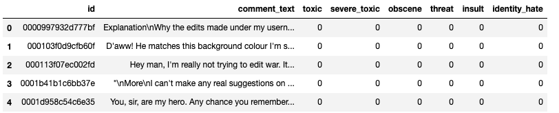
The code snippet shows the first 5 rows of the dataset.

From the dataframe below, the comment_text column is the main input of the data into the machine learning model. According to the dataframe, each class column is shown in binary representation with 1 indicating the matched-class, and 0 being the non-matched class.


The data is removed with the null value or the empty string.

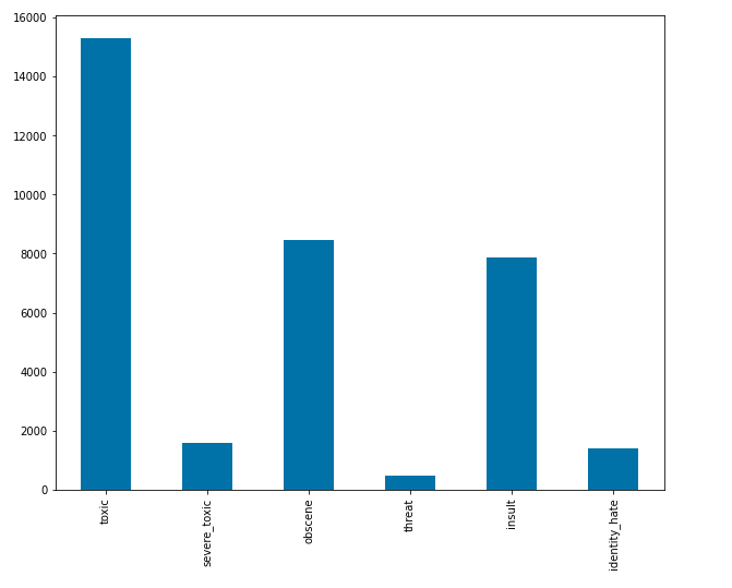
The code cell below demonstrates the comment count plot for each label. The dataframe would be filtered with the 6 labels. Then, the bar plot is shown the count of each class.

From the bar plot below, most comment data are toxic with 9.5%, followed by the obscene and insult classes with 8,449 and 7,877 records respectively. On the other hand, there are the least records in the threat class.


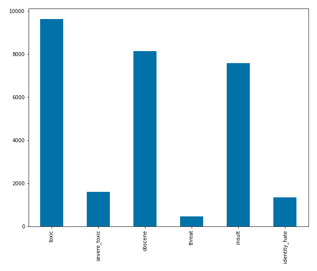
From the count bar chart below, most comments in toxic, obscene, and insult class are multi-labeled. There are 9,628 toxic comments, where obscene and insult comments are around 8,000. On the other hand, there are only 456 comments on the threat class. The comments of multilabel are the least in the threat class.


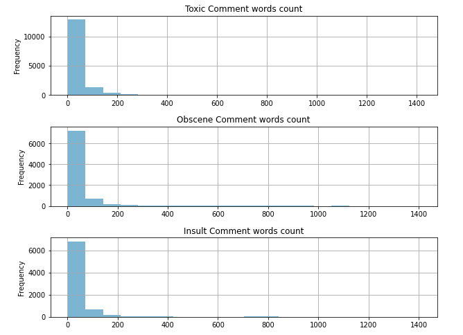
From the words’ count comment histogram, there are around 73.6% comments with the words’ count under 71.5. There are around 32,000 comments ranged from words’ count between 71.5 and 212.5. Then, a few words’ count comments are ranged from 212.5 to 424 with 0.04 comments. On the other hand, there are 4 comments with words count above 1,340.


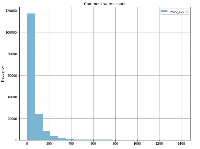
Look into the words’ count of top classes in the comments dataset. In the toxic comments, most words’ count is ranged below 72. Then, there are 11.9% comments’ words’ count ranged from 72 to 213. The highest words count is ranged above 1,340 in the toxic class. In the obscene class, there is around 85.7% of comments’ words’ count fall under 72. There are 10.7 % comments’ words’ length ranged between 72 and 212. There are 3 obscene comments with words length above 1332. In the insult class, there is around 86.4% of comments’ words’ count fall under 72. There are 10 % comments’ words’ length from 72 to 212. There are 2 insult comments with words’ length above 1332. Furthermore, there are 3 multi-labeled comments with the words count above 1332, and those comments are labeled as toxic and obscene.

Keras Multi-label Text Classification Models

There are 2 multi-label classification models introduced with a single dense output layer and multiple dense output layers. From the single output layer model, the six output labels are fed into the single dense layers with a sigmoid activation function and binary cross-entropy loss functions. Each neuron in the last output layer would be one output of six comment labels. The value of the sigmoid function would be between 0 and 1. When the neuron’s value is higher than 0.5, the comment would be classified into that class with a higher probability. There would be 6 dense output layers with the sigmoid activation function.

Single output layer of Multi-label Text Classification

We would introduce the single output layer of the multi-label text classification model in the section. The first step would clean up the text within the created function. In the preprocess_text function, there would be punctuations and numbers removal, single character removal, and multiple spaces removal. The input data is the comment from the comment_text column. X is the list variable containing the cleaned comments after going through preprocess_text function. Y variable includes the output class labels from the comment dataset. There is no further processing on output labels since the labels are already in the one-hot encoding format. Then, the data would be split with 80% of training data, and 20% test dataset. The text input to the model would be the embedding vector. From the text preprocessing, the Keras tokenizer library is implemented with the top 5,000 vocabularies considered. Then, the text would be transformed into sequential integers from the tokenizer library. To have the same vector size of the text in the comment, the words are padded with the length of 200.
There would be additional input text vectors from GloVe word embeddings. The text would be transformed into the embedded vectors through Glove with the Wikipedia input corpus.
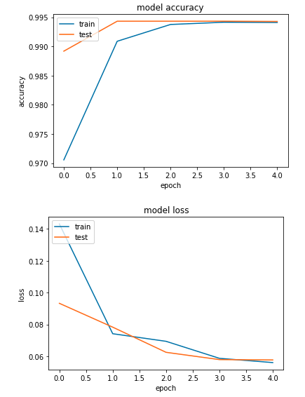
  The model is created in the following script. The model would be composed of one input layer, one embedding layer, one LSTM layer with 128 neurons, and one output layer with 6 neurons while there are 6 output labels in the comment dataset. The parameter trainable=False is used to keep weights from being updated during training. The weights of the embedding layer are input with the Glove embedding. The loss function of the model is binary cross-entropy along with the adam optimizer. The batch size of the model is set with 128, and there is a 20% split on the validation data. The model is evaluated on the test dataset with a test loss of 0.056, and an accuracy score of 99.4%.

The accuracy and loss graphs are shown below. The training accuracy is a bit lower than the test accuracy from the first 3 epochs. Both training and test accuracy scores are growing with more epochs. The test loss is lower than the training loss within 3 epochs. Both training and test loss are decreasing with more epochs.

Keras Text Classification with Multiple Output Layers

There are 6 labels combined in the y variable, and y variable would be split into several labels where each of them is input into each output layer. There would be 6 individual labels in the train and test dataset.  The model is structured with one input layer, one embedding layer, and one LSTM layer with 128 neurons. There are 6 dense output layers, and each layer is for each label in the model. Each output layer will have 1 neuron with a sigmoid activation function which produces a value ranged between 0 and 1. 
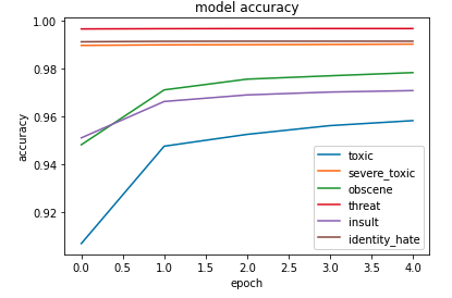
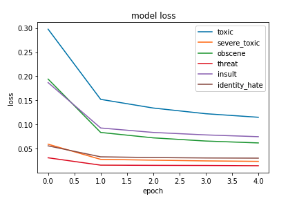
The model result is shown in the graphs below. Top 3 classes such as threat, identity_hate, and severe toxic reach the 99% accuracy rate within the 5 epoches. In addition, the obscene and insult class achieve a 98% accuracy rate. Overall, the performance of the multiple output layers is above 96%. In terms of the loss, the loss of three classes likewise threat, severe toxic, and identity hate is around 0.05, and the loss is computed by the binary cross-entropy.

Conclusion

It is quite common to meet the multi-label text classification problem. In the article, it is introduced with two deep learning approaches for multi-label text classification. One is the single dense output layer with each neuron predicting one label, and the other is a separate dense layer with one neuron for each label. The result from the single output layer with multiple neurons is better than the multiple output layers.

Reference

• Python for NLP: Multi-label Text Classification with Keras
  https://stackabuse.com/python-for-nlp-multi-label-text-classification-with-keras/