Time Series Forecasting of the monthly sales with LSTM and BiLSTM

In this article, it introduces the time series predicting method on the monthly sales dataset with Python Keras model. The article would further introduce data analysis and machine learning.

In this article, you will learn the LSTM and BiLSTM modeling method for the monthly sales dataset:
(1) Introduction
(2) Data Wrangling
(3) Data Transformation to make it stationary and supervised
(4) Building the LSTM model & evaluation

Introduction

Time-series forecasting is one of the major concepts of Machine Learning such as Autoregressive Integrated Moving Average (ARIMA), Seasonal Autoregressive Integrated Moving-Average (SARIMA), and Vector Autoregression (VAR). In the article, we would mainly focus on LSTM, which is considered the popular deep learning method. 
The objective of the monthly predictive sales is to know the future sales and help the business. First of all, we can plan the demand and supply based on the monthly sales forecasts. This helps to know where to make more investment. Then, it is seen as a good reference for the further planning budgets and targets.
The dataset applied in the sales forecasting method is from kaggle. In the training dataset, it contains columns of date, store, item, and sales. There are a total of 913,000 rows from 2013–01–01 to 2017–12–31. Besides, there are 50 items sold from 10 stores with the daily sales. 
The code cell below is to aggregate our data at the monthly level and sum up the sales column. From the aggregation process, the dates are converted into the beginning date of each month.

Data Transformation

The transformations methods are applied for the model predicting method:

• The data would be converted to be stationary if it is not
• Converting from time series to supervised for having the feature set of our LSTM model
• Normalize the data

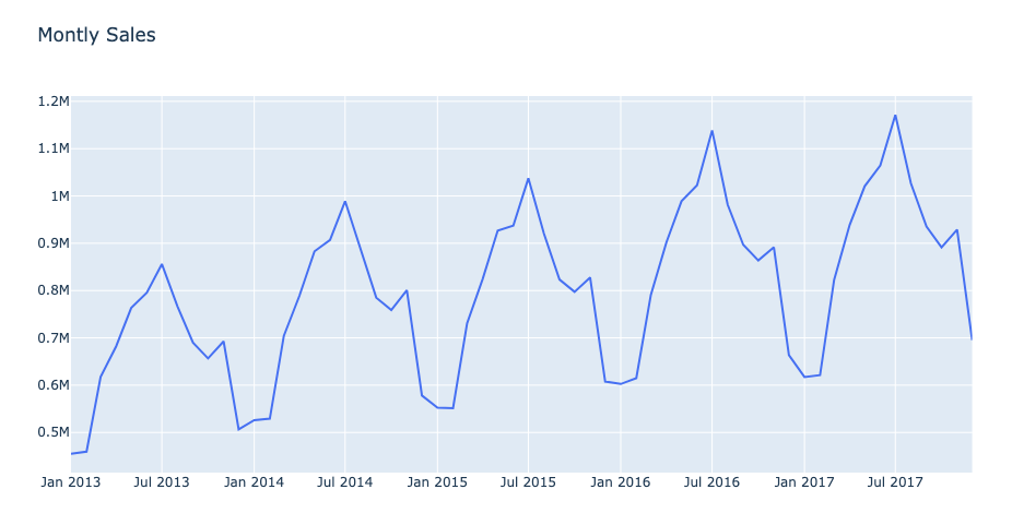
From the monthly sales plot below, it shows that the plot has an increasing sales trend without being stationary. The method applied later is to compute the sales difference compared to the previous month. Then, the model would be built with the features of sales difference. 

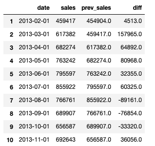
The column of the previous sales contains the sales from the previous month. The diff column is the sales difference between the previous and current month. Without the null value, the beginning month would be February in 2013.

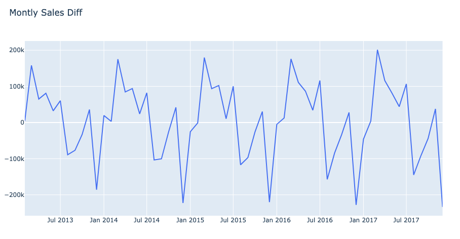
The plot shows the monthly sales difference over the months from 2013 to 2017. The sales difference shows the stationary sales pattern.

Then, the feature set would be made from the previous sales data. The goal is to forecast the next monthly sales from the input of the different sales over the past year. The look-back period is set as 12 and can be varied for every model. The lag features are named as lag_1 to lag_12 columns by using the shift() method.

Adjusted R-squared is to determine whether features are useful for prediction. Adjusted R-squared shows the feature variance from lag_1 to lag_12 for diff. The code cell below shows that the linear regression model (OLS - Ordinary Least Squares) is applied and the Adjusted R-squared is computed. The example shows the variation of the lag_1 to the column diff. The result shows that lag_1 has 3% of the variation. While adding more features, the variance increases from 3% to 98%, which is quite impressive. The model can be built with more confidence after scaling the data. 

Before scaling, the data shall be split into train and test sets. The last six months sales data is extracted to the test set. MinMaxScaler is applied as the scaler. As the scaler, we are going to use MinMaxScaler, which will scale each future between -1 and 1:

Building the LSTM model

The lagged features are generated from the difference between the current month’s sales and last month’s sales. There are 12 lagged features produced as monthly-sales difference through a year. The lagged features would be split into feature and label sets from the scaled dataset. The label for the train and test dataset is extracted from the difference (previous month) sales price. In the time series model, the data is reshaped into 3 dimensions as [samples, time steps, features]. The data input is one-time step of each sample for the multivariate problem when there are several time variables in the predictive model.

There are two LSTM model to compare the performance. One is the LSTM model with an LSTM layer with 4-unit neurons and 1 Dense layer to output the predictive sales. The stateful parameter is set as True when the last state for each sample at index i in a batch will be used as the initial state for the sample of index i in the following batch. On the other hand, the Bidirectional lstm model combines the output from the recurrent layer (LSTM layer) before passing it to the next layer by concatenating. The output number are double at the Bilstm layer. In the Time Distributed layer, it would produce several outputs in a time step. In this example, there is 1 neuron given the time distributed layer so there would be 1 predictive monthly-sales difference from the last layer.

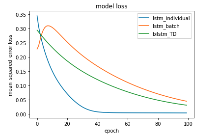
The loss function is mean_squared_error, and the optimizer is adam. The loss of the LSTM model which is trained with the batch data increases through the first 15 epochs. Then, the loss decreases afterward. The loss of the lstm model with batch data is the highest among all the models. However, the loss of the lstm which is trained with the individual data decreases during 35 epochs, and it became stable after 40 epochs. The lstm model with the individual train data is the best, so it is selected to reverse the predictive monthly sales output from the model.


The following code shows that the predictive monthly-sales difference is computed through the inverse transformation for scaling. It goes through the steps as followed.

• Get the predictive monthly-sales difference and is reshaped into 3 dimensions
• Concatenate the 3-d label tensor with other lagged feature tensors
• Reshape the 3-d tensors into 2-d, and they are transformed inversely through the scaler

The transformed prediction is the sales difference of the previous day. Take the transformed sales prediction difference, and add the sales of the previous day. The added value from the output would be the predicted sales at the current date. Then, the data frame is created with the dates and the predictions.

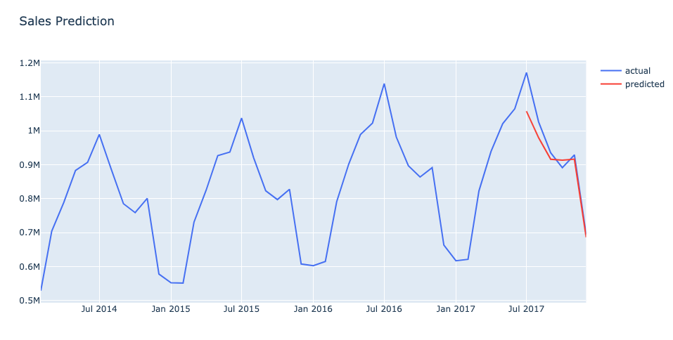
From the plot below, we predict the six-month sales from July 2017 to December 2017. The red line shows the predicted sales value. From August to December in 2017, the sales gap becomes narrow.

Conclusion

• To better predict the monthly sales data, the data would be converted to be stationary if it is not. Then, we convert from time series to supervised for having the feature set of our LSTM model. Adjusted R-squared is to determine whether features are useful for prediction. The higher values of the Adjusted R-squared would indicate that the features are more correlated. Before the model training, the input dataset into the LSTM model is the normalized values.
• In the time series model, the data is reshaped into 3 dimensions as [samples, time steps, features]. The data input is one-time step of each sample for the multivariate problem when there are several time variables in the predictive model. Among 3 modeling approaches, the lstm model with the individual dataset has the best output, whereas the lstm model with the batch data has the highest loss. Since there are only 41 timesteps of training data, the performance of the batch model training method does not produce the optimum result.
• From the predictive-sales transformation process, we get the predictive monthly-sales difference which is reshaped into 3 dimensions. Then, we concatenate the 3-d label tensor with other lagged feature tensors. Afterward, the 3-d tensors are reshaped into 2-d which are transformed inversely through the scaler. Take the transformed sales prediction difference, and add the sales of the previous day. The added value from the output would be the predicted sales at the current date.

Reference

• Predicting Sales
  https://stackabuse.com/python-for-nlp-multi-label-text-classification-with-keras/
• How to Develop a Bidirectional LSTM For Sequence Classification in Python with Keras
  https://machinelearningmastery.com/develop-bidirectional-lstm-sequence-classification-python-keras/